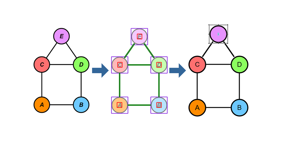
Once a year the yWorks office is alive with a very special atmosphere: The project days. Small groups of developers gather together to work on projects that are not necessarily connected to the everyday work or the core products of the company. This year, four brave developers set out to new lands and tried to parse photos and screenshots of diagrams as actual yFiles graphs without ever having touched computer vision topics before. This is their story.
Motivation
Do you remember the last time you've created a diagram on paper and found yourself re-creating it in a general diagram editor like yEd? This use case isn't that uncommon, because we often sketch out our ideas in form of diagrams during meetings or plan certain processes on the whiteboard. Usually, we want to digitize them afterwards in order to make small incremental changes and insertions or even apply an automatic layout algorithm to clean up the chaotic arrangement.
Slightly easier input images are programmatically generated diagrams, e.g. printed in literature, that have consistent styling across all items. Still it would be great if we could create a digital graph model from this image.
In this project, we try to make a first approach towards this general problem and see whether we can acquire new experiences in the field of computer vision.
General Approach
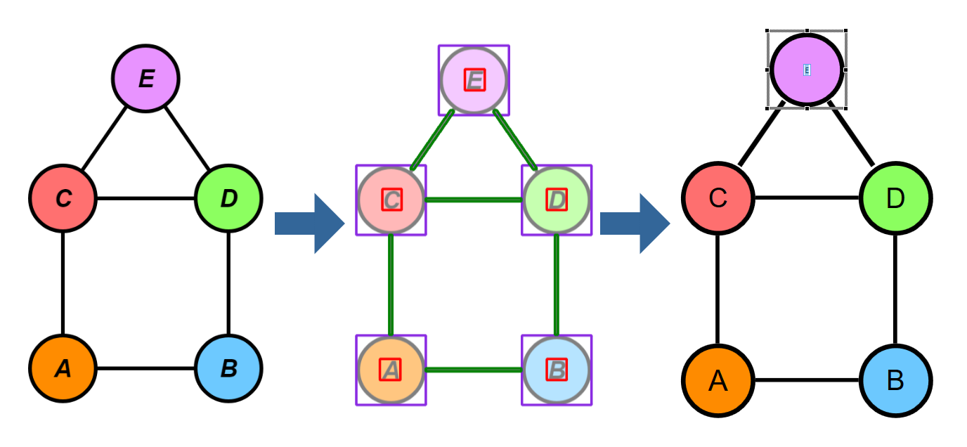
After some research on the topic, we decided to take a shot at it with Python and OpenCV for parsing the image and eventually create JSON output describing the relevant diagram elements with layout and styling information. This output could be easily consumed by any general purpose diagramming library, though in our case, we will build a yFiles WPF application for rendering the parsed diagram.
Processing Pipeline
We decided on a processing pipeline which should give us the flexibility to simultaneously work on separate parts of the project.
The first and basic step is the image segmentation where the image is broken down into disjoint regions of the overall image, each of which contains either a node, or an edge. Those regions can then be further processed independently to detect different features (e.g. color, shape, edge bends, etc.). Of course, the quality of the segmentation step impacts all the subsequent processing on the separate regions.
Segmentation
Given the entire input image, we first need to separate it into node and edge regions, which simplifies the identification of more features in the resulting regions. All subsequent operations are performed based on this initial segmentation which is crucial for the overall result, since elements that haven't been segmented properly will be missing or merged in subsequent steps.
We've explored several approaches here and found that there doesn't seem to be one single approach that works for arbitrary input. Therefore, we kept a selection of segmentation algorithms and chose one of them depending on the current input. The following sections describe the segmentation algorithms we've implemented in more detail. This list is not exhaustive, as we had several ideas for other algorithms that could work better for certain inputs.
Automatic Color-based Segmentation
This segmentation approach tries to distinguish nodes, edges and background based on their color with the requirement that the elements of each category have the same color (which is unique for each category) and with the restriction that we only have three unique colors in the image.
At first, a 3-color quantization step is applied to the image to reduce errors from anti-aliasing or uneven exposure. From the resulting colors, we assume that the most frequent color marks the background, while the second-most frequent color represents the nodes and the least frequent color is the edge color.
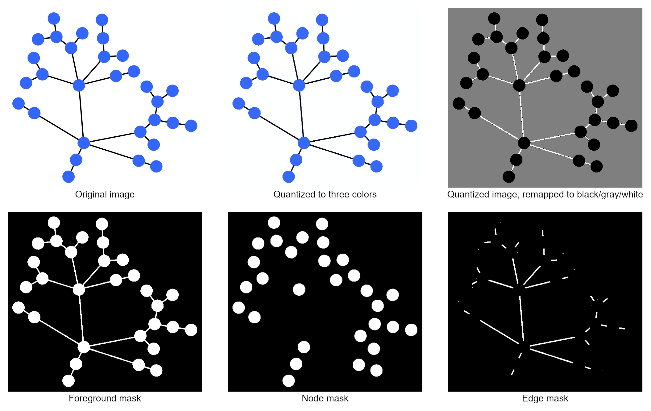
Although this sounds like a pretty strong assumption, it works surprisingly well for many programmatically-generated graphs and also for certain hand-drawn or scanned pictures that share the same traits. If the node and edge colors are too close, anti-aliasing sometimes causes artifacts near the border of nodes and edges that are wrongly classified. Such artifacts can later be removed due to their implausible size.
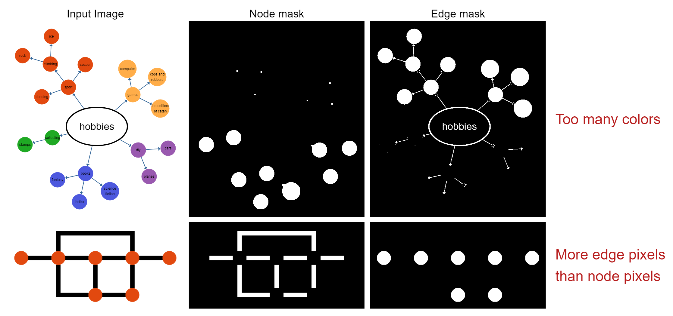
However, the obvious drawbacks are that it doesn't work for images where nodes may have different colors, or are not filled. The segmentation also fails if the ratio between background, node, and edge pixels is not as expected, e.g. if there are many edges, and rather small nodes, the edge color will be incorrectly assumed to be the node color based on its frequency in the image.
Morphology-based Segmentation
The second approach to the segmentation works with morphological transformations on the input image. Morphological transformations change a binary (i.e. black and white) image globally according to certain rules.
The first step for this is to convert the input image to grayscale and subsequently to black and white to be able to use morphological transformations. Then, we find the outermost contour in the image and assume this to be the foreground (i.e., the graph). This contour is used as the initial mask.
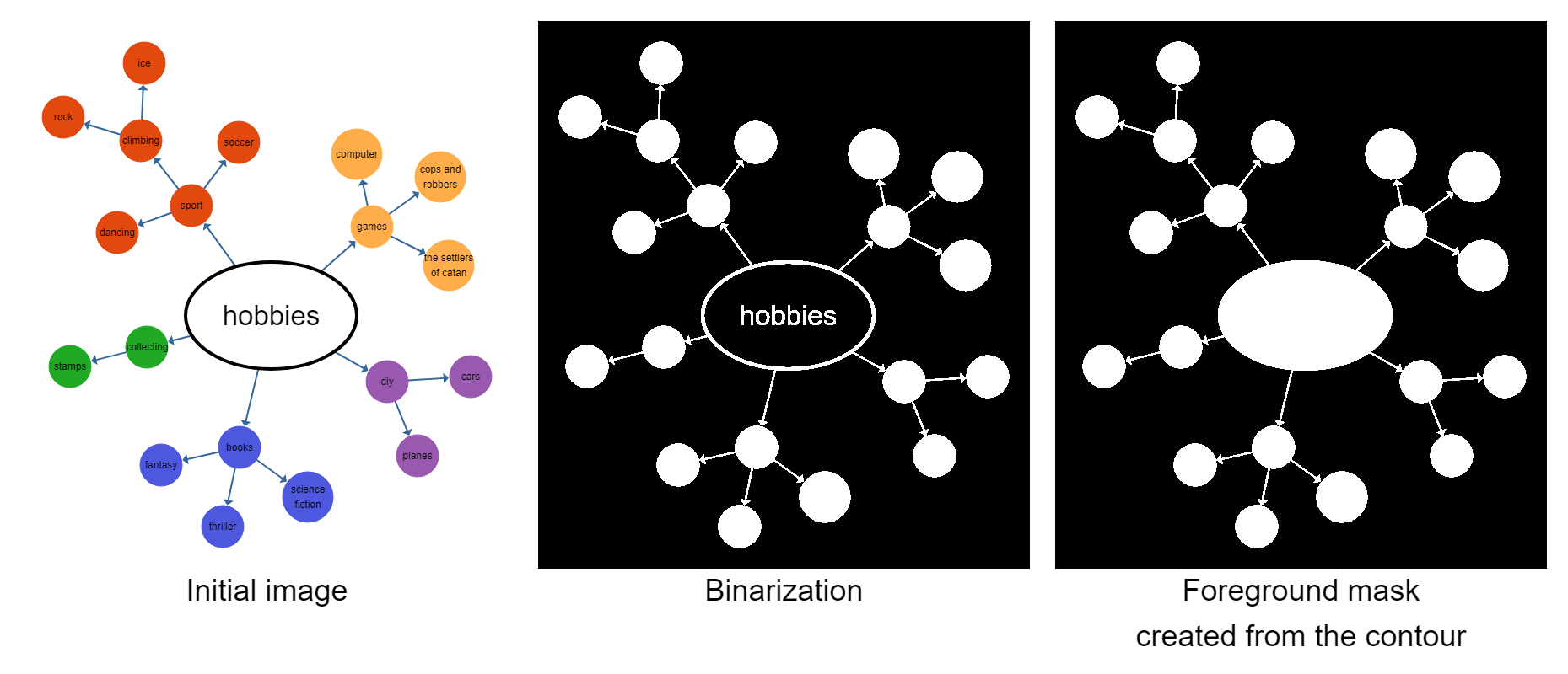
We then try to remove edges in the image by running multiple erode passes on this image. Erosion is an operation that removes pixels from the outside edge of shapes. This implies that thin features, like edges, eventually disappear after multiple erode steps, while nodes will get smaller, but still remain in the image. After all edges have disappeared, we reverse the process with dilation, which adds pixels on the outside edge of shapes, to ensure that the nodes are roughly as large as they were in the beginning. We can then run OpenCV's findContours() on the image to detect our nodes. Given the nodes' contours, it is trivial to create an edge mask in which we can detect the edge regions for our segmentation.
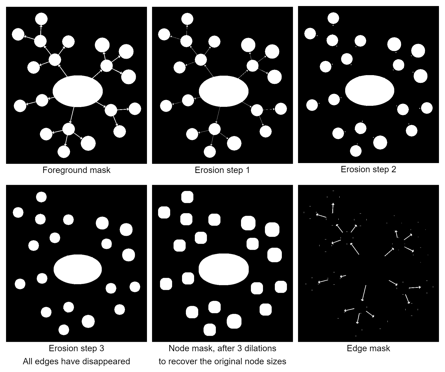
A major challenge in this approach is to detect how often we need to erode the image until the edges are removed. The number of erosion steps depends on the thickness of edges, and we employed a heuristic where we observe the number of contours in the image for each step. At some point, the image will disconnect into several new contours and multiple subsequent erosions won't significantly change the overall number of contours. This is assumed to be the point where the edges disappeared and the nodes on both ends of the edge now form their own individual contours. This heuristic has been introduced to be able to segment images where the edge thickness is similar throughout the image, but can vary from one image to the next, without having to adjust constants in the code.

This segmentation approach works well for diagrams where the color-based segmentation is not suitable, for example when nodes and edges have the same color. However, it fails for diagrams where the edge thickness differs strongly due to the adaptive cut-off for the erosion steps. In those cases, certain regions of the diagram won't disconnect and, therefore, be considered as an entire node region, which causes problems for the node detection in this area. Unfilled nodes with just an outline present a challenge because we cannot separate foreground and background globally by color. Instead we must use the surrounding contour, which requires that edges in the graph cannot enclose a background region. This would then be detected as a node instead
Manual Marking of Nodes
We had a fair number of test images we wanted to use — especially for later stages of the pipeline — that couldn't be segmented by either of the other two approaches. We added a fairly simple segmentation approach where the user marks each node by clicking on it. Nodes are then detected by taking the color at that point and finding the whole region around it. After all nodes have been marked, the image is converted to black and white, nodes are removed from that image, and the remaining contours are detected as edges.
This works well for graphs where the nodes have many different colors (negating the automatic approach), or regions enclosed by edges (preventing the morphological approach from working). An obvious drawback is that it's tedious when there are many nodes. Furthermore, edges cannot have the same color as their adjacent nodes, because otherwise the edge would be detected as part of the node.
Node Labels
Besides the general segmentation in edges and nodes, we also detect label regions within nodes.
Given the already detected node regions, label detection is rather simple, because running OpenCV's findContours() on a threshold image of the node region provides not only the outline contour, but also all nested contours. Any nested contour marks a character inside the node. The bounding box of these nested contours then builds the label region.
There are several problematic aspects to this approach. First, the label needs to be enclosed by the node, otherwise the label will be clipped at the node's bounds. Also, the font to node fill color contrast needs to be large enough so that it does not get lost in the image threshold and the node needs to have a solid fill and no empty holes that may be detected as inner contour.
Although these are quite some limitations, there are still many use cases that fulfill the requirements with which the labels can be detected properly. In the resulting graph model, the labels can then be either used as clips from the original image or an actual text label can be created by applying OCR.
Node Detection
Based on the image clip that is defined by the node region provided by the segmentation, we try to further identify properties for the nodes. The goal is to detect the main features that are characteristic for a node, i.e. the shape (rectangle, triangle, ellipse, ...) and the color, where we want to detect the fill color, the outline stroke as well as the stroke thickness.
Node Shape Detection
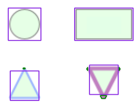
In this step, we want to determine the shape of the each given node region. The pre-processing in the pipeline already provides an outline of the contour in the node region, so the challenge in this step is to decide whether the given contour is a rectangle, triangle, ellipse etc. The contours are not normalized in any way, therefore we need to consider the different sizes as well as to determine whether they are rotated or not, because we also want to detect, for example, whether a triangle is upside down or not.
In general, OpenCV comes with a matchShapes() function with which a similarity score of two given contours can be calculated. This function is scale and translation invariant. However, it is also rotation invariant which is why we decided to implement another approach for this task.
What turned out to work quite good is creating specific shape masks with the same size for each separate node region and shape that we want to detect. With these masks, we calculate the difference between the actual contour mask given by the segmentation and these shape masks. The similarity then correlates with the non-zero entries after bitwise XOR combination of the inverted shape mask and the contour mask of the node itself. The more non-zero entries this bitwise XOR combination yields, the better the reference mask matches the original contour.
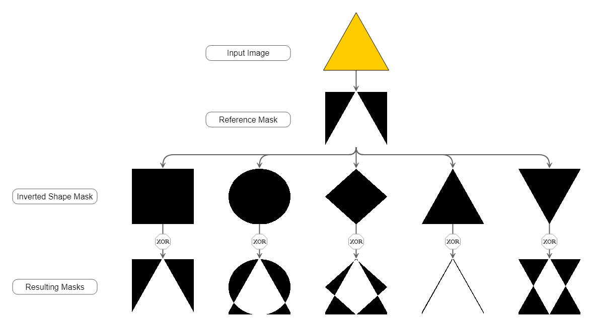
Although this approach requires to re-create all reference masks for each node, the performance still turned out to be good. The mask creation and bitwise matching are cheap operations and at least as fast as using the built-in matchShapes() method.
Fill and Stroke Detection
Similar to the shape detection, the color is one of the most important properties of a node when creating a graph from an image.
To detect the fill color of the node, we decided to use a k-means clustering with k=10 on the color of the pixels within the node contour but ignoring the label region if there is any. The cluster with the largest number of pixels determines the main fill color.
This simple approach turned out to work quite well as long as the node region does not contain a large number of anti-aliasing pixels. However, for small ellipses it often produced a mixed color depending on the ellipse's stroke because of the anti-aliasing pixels on its outline.
Now that we have our k-means clustering for the color, the most obvious approach for the stroke color would be to just use the second largest cluster that is not the background color. But as it turns out, this only works for very specific shapes and sizes and thus often yields wrong results.
Our approach for detecting the stroke color is to generate one pixel slices from the contour of the node. We iterate from the outside to the inside and create an even tighter slice for each iteration. During the iteration, the main color for each slice is picked using k-means clustering. Once this color is similar enough to the fill color of the node, we stop the iteration and know that the pixels of all slices build the stroke outline of the node. Therefore, one last k-means color clustering can be applied to those pixels in order to get the stroke color.
This approach can also be applied inside-out when the given node contour does not contain the stroke outline, which may be the case depending on the initial segmentation approach.
Another benefit of this iterative approach is that it implicitly yields the stroke thickness as well, since it is the iteration count for generating the one pixel slices until the stop condition is met.
Edge Detection
Of course, a graph usually does not consist only of nodes but of edges, too. We already get regions for each individual edge from the segmentation. We now need to figure out where an edge starts and ends, as well as how its path looks like. Later on, we also try to detect visual features so that the resulting edge looks as close to the original image as possible. These include the exact positions where the edge attaches to the node (the port positions), the edge thickness, color and direction.
Edge Geometry
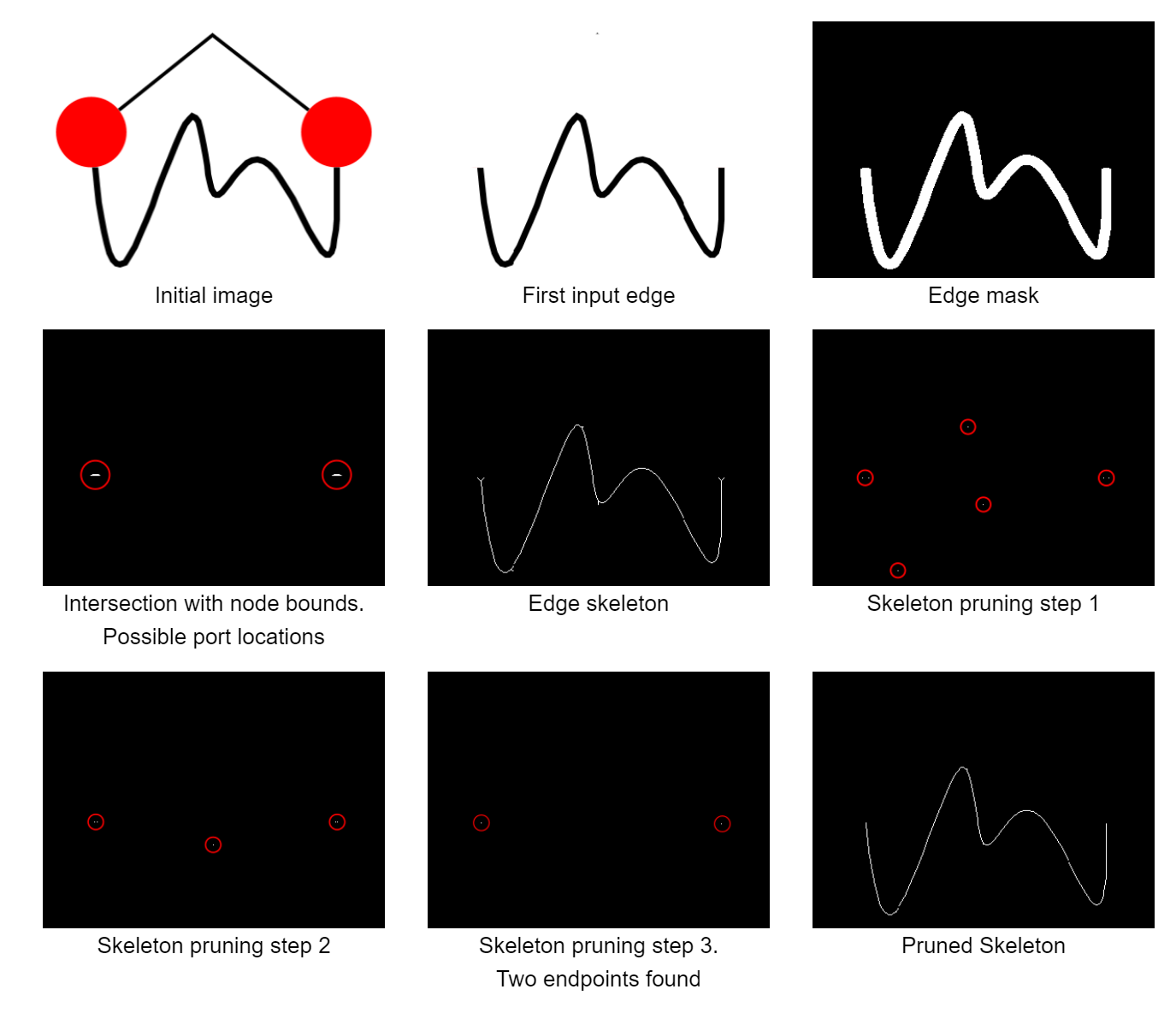
To start with, we need to convert the edge region, which encompasses the whole edge path, to something that is easier to work with. To this end, we perform skeletonization by morphological thinning. This skeleton retains the basic shape of the original input and also stays connected, just reduced to an one-pixel wide line. This makes it easy to detect certain features, such as end points of a line, corners, or crossings, simply by looking at a pixel and its immediate neighborhood. One remaining problem is that - especially for thicker edges and arrowheads - there are a lot of branches, or spurs, leading off from the core skeleton. We prune those away by successively identifying end points via a hit-and-miss transform and removing them, until only two end points remain.
Those two end points are then matched to their closest node regions to determine the two end nodes. Furthermore, since we have two end points and we know that the whole line is connected, we can just walk along the neighboring pixels from one end point to the other to obtain the edge path. Of course, this path has a bend point at each and every pixel, so we apply the Douglas-Peucker algorithm to approximate a polygonal line that better matches the original image.
We also need to figure out the port positions, where the edge attaches to the node. Due to the pruning step that we applied earlier to remove the spurs and retain only two end points, we've also pruned away the actual end points of the line, which are now further away from the node. This isn't much of a problem for determining the end nodes, but it means that we've lost part of the edge path near the node and cannot easily determine the actual position on which it was attached at the node. To remedy this, we've started with just the two end points from earlier and used morphological dilation to grow them until we find the intersection with the nodes. This is somewhat error-prone and not ideal, and more attributed to our inexperience and and the fact that we didn't have a better idea for the earlier stages as well. More on that below when we compare our approach to existing approaches (which we've found after settling on this approach).
Edge Styling
To further capture the fidelity of the detected edges, we also detected two main features to make them look more similar to their original counterparts from the input: Color and thickness. The color is determined by taking the dominant color along the edge's skeleton. This skeleton is completely inside the detected edge region and, thus, only yields pixels belonging to the edge. This works well for many edges, but can result in the wrong color when the edge is very thin and anti-aliased, since the algorithm picks up more anti-aliasing pixels than pixels of the actual edge color. Thickness is determined by taking the number of steps required for the skeletonization in the beginning. The process of obtaining the skeleton takes away pixels from the outside of the shape until nothing else can be removed without breaking the shape, so the number of those steps is roughly half the thickness of the edge in pixels. Due to some inaccuracies on how we've implemented skeletonization this doesn't fit exactly, so a better factor has been determined empirically. We've also included a heuristic to detect whether the original edge path was curved and apply a smoothing step to the edge style on the yFiles side to mimic the original curvature.
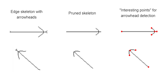
Directed graphs have a direction for each edge, usually signified by an arrowhead on the target end of the edge. To detect those arrowheads we start with the original skeleton, where arrowheads are represented by two long spurs near the target end of the edge. We then prune away the shorter spurs again and see whether we end up with a cluster of exactly three end points near one end of the path. This is then interpreted as the arrowhead and defines the edge direction.
Showcase
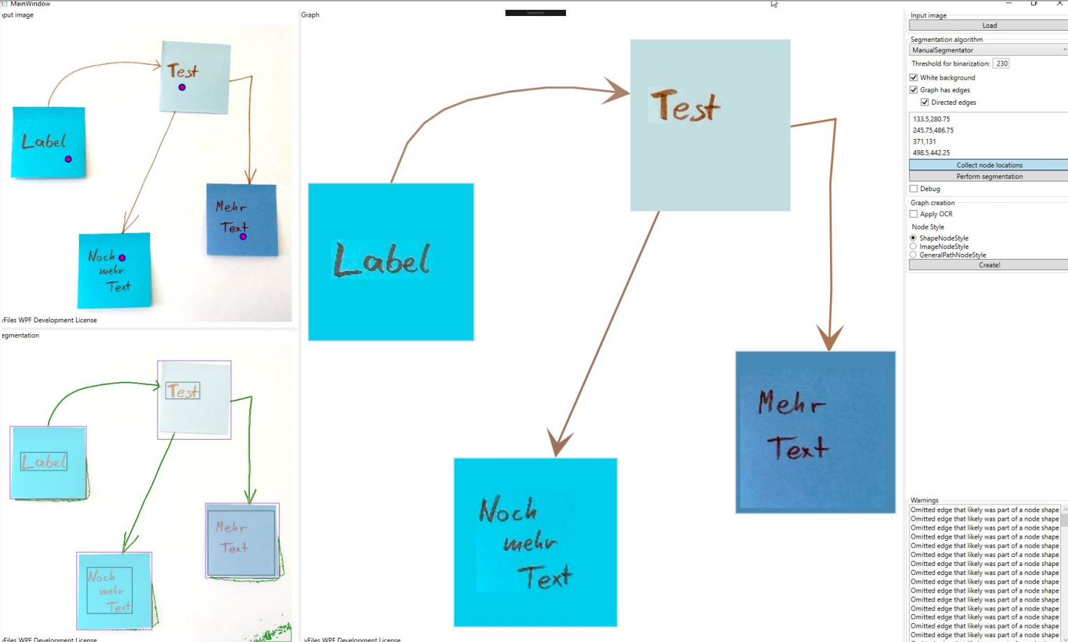
In this section, we want to show some of the results for different input images. To test our different approaches, we built a small C# application where we could experiment with the algorithms on different inputs. The application itself is quite barebone and provides three separate panes. In the top left pane, the input image is displayed. The bottom left pane shows the segmentation regions that are overlaid over the original image. The larger right pane is an actual yFiles WPF component where the the parsed graph is created and displayed, meaning that all the items that are displayed in this pane are graph model items.
Click the image to open the album.
State of the Art
During our work on the project we encountered two existing publications tackling the same problem: Optical Graph Recognition by C. Auer et al. (2013), and Optical Edge Detection by R. Opmanis (2018), which improves edge detection compared to the earlier paper. Surprisingly for us, our approach was fairly similar to what the actual professionals used, even though we had very little prior experience in Computer Vision. Major differences between the existing publications and our approach were the scope of the work and the areas on which we decided to invest time and effort. Mainly, the existing approaches concentrated on getting the graph structure correct. Our approach, being more visually driven, aimed at improving the fidelity of the recognized graphs, i.e., shapes, colors, labels, and edge directions. Those are topics often hinted at in the publications as being useful to pursue further.
Those differences naturally result in different features and drawbacks for each of the approaches. The 2013 paper by C. Auer et al. employs a morphological segmentation approach that requires images of graphs with filled nodes and edges to be significantly thinner than the node size. Edge detection is handled by also identifying crossings and in many cases correctly recovering the original path of all edges, including those that cross each other. Their approach to edge detection also recovers port locations faithfully and thus, detecting the wrong source or target node for an edge is next to impossible. The 2018 paper by R. Opmanis uses a different approach to edge detection and improves detection of crossing edges as well as allowing dashed edges.
Our approach did not attempt to handle edge crossings, instead we've invested more time in different segmentation approaches, which allows to lift some of the restrictions of the earlier approaches. We've also conflated the segmentation step with the pre-processing step, which enables segmentation approaches based on color. Under certain conditions we can correctly segment images with outlined (instead of filled) nodes, and our edge detection can also handle wildly varying edge thicknesses. However, both of those improvements place additional constraints upon either the colors or the graph structure of the input. Our edge detection, as mentioned, is less sophisticated and sometimes has problems with identifying the right source or target node as well as the exact port locations. This is mostly due to us not re-evaluating our choice of algorithm and finding the mentioned papers rather late in our development process. On the other hand, we are able to detect edge color, thickness, and direction via arrowheads fairly reliably in many cases. For nodes, we also have approaches for detecting the node shape, color, and outline. Color detection for both fill and strokes works well in many cases, but has proven to be unreliable with very thin features and anti-aliasing, where the apparent color to a viewer is not the one we can recover.
Concluding, both the 2013 paper and our approach share a number of similarities, mainly in how morphological transformations are applied. By combining the existing approaches with our improvements to fidelity as well as with what we learned, we're sure the overall result in optical graph recognition can be further improved.
Conclusion and Future Work
We believe that our approach can be merged well with existing approaches to improve several aspects on both sides. The mentioned existing approaches generally have better recognition of the graph structure, including edge crossings. In contrast, our approach offers better fidelity that results in graphs that look very much like the input, including labels, shapes, and colors. For the task of digitizing a graph from an image and working further with it, styling information is very nice to have as part of the conversion process instead of having to add it manually afterwards.
Of course, our own algorithms are very much at a prototype stage right now — due to limited time — and could certainly use improvements in many areas. Many stylistic aspects we detect are fraught with edge cases and smaller problems: edge thickness can be unreliable to detect, colors of thin edges or outlines can be subtly wrong due to anti-aliasing, shape detection can only detect a very limited set of shapes right now, etc. Perhaps the part that could use most improvement would be the segmentation, where small improvements could already result in vastly better segmentation. The hard-coded three-color quantization for the automatic color-based segmentation is an obvious limitation that can be removed to allow for graphs that have multiple node colors. Manually aiding the segmentation by either preparing a good background/foreground mask or correcting segmentation errors are also ideas that would greatly help real-world usage of such an approach, as segmentation errors will always happen, but some of them result in graphs that are hard to correct. Especially photos pose a unique challenge in that uneven exposure can make correct segmentation difficult with our current approaches.
On the other hand, there are already many cases where the current version provides very good results - see the provided gallery for examples.
What do you think about the topic and our results? Let us know! Just leave us a message in the social media or using our contact form.


